The
APCH model = Age Period Cohort and hysteresis
Louis Chauvel
Site : www.louischauvel.org/apchex
email : chauvel@louischauvel.org
This web page intends to present the STATA “ssc install apch” ado file, its
methodological background and some examples.
1. Problems:
The first problem
with APC models is the lack of stability of the “detrended cohort estimates”
DCE estimates (see 2. Methods): whether nominal or real mages are estimated,
most APC models (including APCIE) offer different estimates. The second and the
worst problem is the question o the stability of the cohort effect over life
course. We know some empirical curves of age and period data (ex: mortality in
2. Methods:
Please download the pdf: www.louischauvel.org/apchmethodoc.pdf where the main concepts are presented with
the model itself.
In this simulation dataset www.louischauvel.org/apchexb.dta in STATA
format, we have several variables r7 r3 r1 h0 mf1 mf2 mf4 that
express different degrees of APC with resilience (r7 show strong waves at age 20 which are absorbed at
age 65) to Mathew effect
(mf4, little fluctuation at age 20 increasing to age 60). The variable h0 is a
configuration of stable APC with (almost perfect) hysteresis. The APC-H makes the difference between these
examples when APC_IE and other models can not.
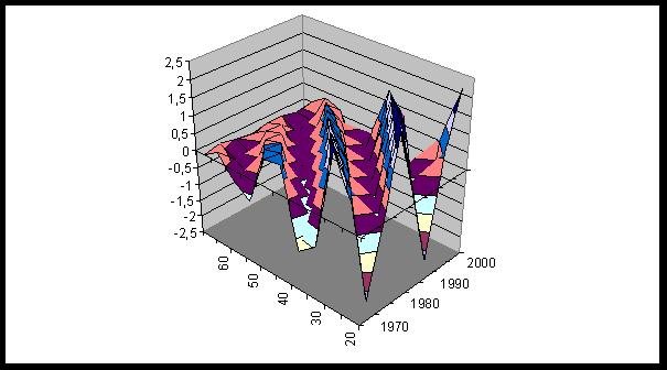
Figure3.1: shape
of r7: simulation of a complete reduction of a cohort effect from age 20 to age
60
The commented do file:
http://www.louischauvel.org/apchex1.do
The value of hysteresis coefficient and reduction of standard deviation
of cohort effect from age 20 to age 65
|
|
Hysteresis |
|
* r7 |
-.9029455 |
|
* r3 |
-.3805228 |
|
* r1 |
-.1204302 |
|
* h0 |
.0002473 |
|
* mf1 |
.1203507 |
|
* mf2 |
.2493086 |
|
Mf4 |
.5184382 |
Figure3.2: shape
of cohort coefficients of r7 after APC_IE
Figure3.3: shape
of cohort coefficients of r7after APCH
4. Second
example: a cohort based variable: veterans
See the do file:
www.louischauvel.org/apchvet.do
[here is an extract of the Ipums
US census and ACS 1980-2010, Steven Ruggles, J. Trent
Alexander, Katie Genadek, Ronald Goeken,
Matthew B. Schroeder, and Matthew Sobek. Integrated
Public Use Microdata Series: Version 5.0
[Machine-readable database].
The status of veteran is deeply connected to birth cohorts. About 45% of
the male population born in 1947 was drafted for the Vietnam War while less
than 10% of those born before 1940 or after 1955 were. Wars are deep contexts
of cohort effect formation and it is why APC analysis of veterans make sense,
but more as a test of a cohort method than as a plan to make new discoveries.
The first step here is to test the apch model
on Vietnam war veterans (viet=0/1)
in a logit APC-H model. We have to add a random 1% of
veterans in the whole population so that we avoid the zero-cell problems of the
logit-APCH method.
The first part of the listing generated by www.louischauvel.org/apchvet.do
gives the APC-D (detrended) list :
The contextual variables give significant elements, first for gender (!)
then for ethnicities: drop outs, Hispanics, other races (that are social groups
specific of a more or less recent entry in the
*********************
* apch version 1.6
*
*********************
*******************************************
####### 1st APC Detrended model #######
*******************************************
Iteration 0: log pseudolikelihood
= -1.304e+08
Iteration 1: log pseudolikelihood
= -1.061e+08
Iteration 2: log pseudolikelihood
= -1.051e+08
Iteration 3: log pseudolikelihood
= -1.051e+08
Iteration 4: log pseudolikelihood
= -1.051e+08
Generalized linear
models No. of obs =
569544
Optimization : ML Residual df =
569522
Scale parameter = 1
Deviance = 210238116.9 (1/df) Deviance = 369.1484
Pearson =
1078990324
(1/df) Pearson
= 1894.554
Variance function: V(u) = u*(1-u) [Bernoulli]
Link function : g(u) = ln(u/(1-u)) [Logit]
AIC = 369.1342
Log pseudolikelihood
= -105119058.5 BIC = 2.03e+08
( 1) [viet]coh_1920 + [viet]coh_1930 + [viet]coh_1940 +
[viet]coh_1950 + [viet]coh_1960
+ [viet]coh_1970 = 0
( 2) - 5*[viet]coh_1920
- 3*[viet]coh_1930 - [viet]coh_1940
+ [viet]coh_1950 + 3*[viet]coh_1960
+ 5*[viet]coh_1970 = 0
( 3) [viet]age_0030 + [viet]age_0040 + [viet]age_0050 +
[viet]age_0060 + [viet]age_0070
= 0
( 4) - 4*[viet]age_0030
- 2*[viet]age_0040 + 2*[viet]age_0060
+ 4*[viet]age_0070 = 0
( 5) [viet]per_1980 + [viet]per_1990 + [viet]per_2000 +
[viet]per_2010 = 0
( 6) - 3*[viet]per_1980
- [viet]per_1990 + [viet]per_2000
+ 3*[viet]per_2010 = 0
------------------------------------------------------------------------------
| Robust
viet
| Coef. Std. Err. z P>|z|
[95% Conf. Interval]
-------------+----------------------------------------------------------------
coh_1920 | -.9911264 .0231308
-42.85 0.000 -1.036462
-.9457908
coh_1930 | -.2940784 .0235157
-12.51 0.000 -.3401685
-.2479884
coh_1940 |
1.116804 .0157177 71.05
0.000 1.085997 1.14761
coh_1950 |
1.660922 .0147736 112.42
0.000 1.631966 1.689878
coh_1960 | -.5403088 .0237761
-22.72 0.000 -.5869092
-.4937085
coh_1970 | -.9522118 .0237156
-40.15 0.000 -.9986934
-.9057301
age_0030 |
.0299572 .0099417 3.01
0.003 .0104718 .0494425
age_0040 | -.0185362 .0118197
-1.57 0.117 -.0417023 .00463
age_0050 | -.0190457 .0131086
-1.45 0.146 -.0447381
.0066468
age_0060 |
-.026129 .0130447 -2.00
0.045 -.0516962 -.0005618
age_0070 | .0337536
.010875 3.10 0.002
.0124391 .0550681
per_1980 |
.0123413 .0076728 1.61
0.108 -.0026972 .0273798
per_1990 |
-.036707 .0112705 -3.26
0.001 -.0587967 -.0146172
per_2000 |
.0363901 .011445 3.18
0.001 .0139583 .058822
per_2010 |
-.0120244 .0077585 -1.55
0.121 -.0272308 .0031819
rescacoh |
-.6508414 .0385203 -16.90
0.000 -.7263398 -.5753431
rescaage |
.0344258 .0125806 2.74
0.006 .0097683 .0590834
hispan |
-.2357637 .0298863 -7.89
0.000 -.2943397 -.1771877
aa |
-.0499998 .0222951 -2.24
0.025 -.0936974 -.0063021
sex |
-2.491538 .0198973 -125.22
0.000 -2.530536 -2.452539
orace |
-.4442171 .0320169 -13.87
0.000 -.5069691 -.381465
_Ieduc_5 |
.3613721 .0492375 7.34
0.000 .2648683 .4578759
_Ieduc_6 |
.9193302 .0272782 33.70
0.000 .8658659 .9727944
_Ieduc_7 | 1.14054 .0298243
38.24 0.000 1.082086
1.198995
_Ieduc_8 |
1.232906 .0317742 38.80
0.000 1.17063 1.295183
_Ieduc_9 |
.7301133 .0308066 23.70
0.000 .6697335 .7904931
_Ieduc_10 | .6832632
.031855 21.45 0.000
.6208284 .7456979
_cons | -.8828439 .0321608
-27.45 0.000 -.945878
-.8198098
------------------------------------------------------------------------------
hystecoh
| -.0142909 .0151769
-0.94 0.346 -.0440371
.0154553
For our purpose, the most important is the cohort effect and the H
coefficient, not significantly different to zero.
------------------------------------------------------------------------------
hystecoh
| -.0142909 .0151769
-0.94 0.346 -.0440371
.0154553
------------------------------------------------------------------------------
Figure4.1: shape
of cohort coefficients of
In order to test the capacity of the APC-H
model to detect decrease of the cohort ehhect over
life course, we simulate data having decreasing veteran statuses over age-span.
Formally, this is equivalent to a progressive transformation of veterans in
non-veterans (loss of status of veteran) with age (see the syntax). We also add
a 1% random veteran status so that the logit
estimation is faster than with almost 0 cells in some cases.
The general shape of the results of the APC-D
model is almost unchanged (evenb if the cohort effects
are smaller, given the transformation we gave to the data. The main change
pertains to the H coefficient which is significantly lower than zero now.
------------------------------------------------------------------------------
hystecoh | -.1247373
.0184565 -6.76 0.000
-.1609114 -.0885632
------------------------------------------------------------------------------
(just notice that H=-
5. Third example: education
Education is, in the
set of common variables, one of the most influenced by birth cohort. The period
of entry in the age of choice between following education or
finding one’s independent life is strategic, in terms of opportunities or
limits.
www.louischauvel.org/apchcpseduc.do
[here is an extract
of 1975-2010 (each 5 years) March CPS extracts source IPUMS, see: Miriam King,
Steven Ruggles, J. Trent Alexander, Sarah Flood,
Katie Genadek, Matthew B. Schroeder, Brandon Trampe, and Rebecca Vick. Integrated Public Use Microdata Series, Current Population Survey: Version 3.0. [Machine-readable database].
These data show the
extreme acceleration in educational resources of the cohorts born in early baby
boom (circa 1950). David Card (xxxx) and Robert Mare
(xxxx) have documented this singularity; the first
one insist in the Vietnam war context that increased
the incentive to follow education, and the second one on the composition
effects of immigration.
Figure5.1: % of BA degree owners (or higher) at
age 45 by birth cohort
When we control by
usual contextual variables, the APCH model shows the specificity of the early
baby boom. These specific traits has been largely commented (xxx)
Figure5.2: shape of cohort coefficients of BA
degree owners (or higher) in the
The value
and 95% CIs of H-coefficient show that the
educational differences are durable; since H is very close to zero, this means
that educational inequalities by birth cohorts are durable.
------------------------------------------------------------------------------
hystecoh | .0025754
.0862099 0.03 0.976
-.166393 .1715437
------------------------------------------------------------------------------
The intensity of the cohort fluctuations for MA
owners is even stronger, and it is amazing that these gaps have received so
modest interest in the sociological literature. For MA owners, a part of the
gap is absorbed over life course (H=-.16), that is significant. This trend of
slight hysteresis could be due to the fact that cohorts with lower achievements
in terms of Ma degree can (partially) catch up later.
------------------------------------------------------------------------------
hystecoh | -.1537173
.0505355 -3.04 0.002
-.252765 -.0546695
------------------------------------------------------------------------------
Figure5.3: % of MA degree owners (or higher) at
age 30, 40 & 50 by birth cohort
Figure8: shape of cohort coefficients of MA
degree owners (or higher) in the
Apart the case of Ma owners with logit specification, all the other models of educational
achievement show no hysteresis index below 0. With a linear specification (not logit), H =+.02, not significantly different to 0.
------------------------------------------------------------------------------
hystecoh | .0206885
.0520695 0.40 0.691
-.0813659 .1227429
------------------------------------------------------------------------------
The linear specification of the model involving
the educ variable as an ordinal variable of
educational level provides similar H=0 result.
------------------------------------------------------------------------------
hystecoh | -.0318595
.0321955 -0.99 0.322
-.0949616 .0312425
------------------------------------------------------------------------------
This means that birth cohort is an important
parameter of inequality of distribution of education, since the context of
educational development between age 17 and 23 is of major importance for
individual’s opportunities. More precisely, the cohorts born in the late
1940’s, beginning of the 1950’s, have benefited from exceptional opportunities
for havin,g longer
education. A major aspect of Age-Period-Cohort specificities in the
Here is also an example of the limits of the
Yang’s and colleagues apc_ie
(intrinsic estimator) model. The aim of the ie is to
provide a “per se” optimal age, period and cohort trend. When we make use of
the apc_ie model for BA or higher owners, education
seams to increase with age and to decrease with period.
Figure5.4: shape of age, period and cohort
coefficients of BA degree owners (or higher) in the
In the general case, the linear trends of the
age, period and cohort coefficient can not be interpreted easily and appear
more as technical intercepts than as meaningful results. It is why we must
prefer the detrended approach, where the real focus is driven to the shocks
below or above the linear trends.
6. Fourth example: economic prestige of
occupation and education
We are interested
here by the socioeconomic achievement in terms of occupations of different
birth cohorts before/after control by education.
www.louischauvel.org/apchcpsprestige.do
We want to avoid here
the risks of tautology: most prestige scales include education as a determinant
of prestige in parallel with income/earning positions. If cohorts with higher
educational level perform better in terms of socioeconomic indexes (where 50%
of the score is based on education) would not be convincing to show the
inequalities of achievement of cohorts. This is why we create an economic scale
of prestige of occupation. In order to have a non-educational prestige, we
consider the parameters of occupation groups in the coding of 1990 (see IPUMS)
of the regression of the logged income by occupation, race, hispanicity
and gender. In this scale, education is not the reference of the construction.
The score is standardized; we provide also a scale where non-employed population
received the score predicted by a regression on education, race, hispanicity, sex.
The scale of economic
prestige shows that cohorts born in the 1950’s enjoy better economic positions.
Figure6.1: Cohort diagram (X axis = birth
cohort; Y axis=prestige; cure=age groups) for the male population
The descriptive
cohort analysis of the prestige scores show the rupture of the cohort born
after 1950. For the male population, at a given age, the cohort progress in
prestige stalls and reverses after birth cohort 1950; for the female
population, we notice very slow growth after the cohort born in 1950 when the
trend was much faster before. In general, these curve means convergence between
male and female population.
But these results are
simply descriptive. Two models are proposed here, the first with controls of
gender and ethnicity, but with no control of education. A second model will
include education (but we present this one for male and female populations
separately).
The APC-H with
controls of ethnicity and gender detects a huge cohort effect with a strong
peak for the cohorts born circa 1950. When it is compared to the cohort
dynamics of education, this is not a complete surprise. This non-linear trend
goes with a H-index non significantly different to
zero. This means the gaps between cohorts are stable along life course. The gap
between the most and the least advantaged cohorts is of .135, that is lower but
of the same scale of gradient than gender gap circa .20.
Figure6.2: shape of cohort coefficients of
occupational prestige model with ethnicity and gender no education
It is interesting to
process separately male and female population with the introduction of the
control by education. In both case, when standard deviation or max minus min are
measurements of cohort inequalities, for both male and female, when education
is taken into account, the cohort gaps are reduced to one third. The shape of
the cohort is also very different. Most of the peak in prestige distribution
comes from the educational peak of the cohort 1950. However for male, some
cohort gaps remain significantly different to 0. Surprisingly, for male, the cohort born in 1955 faces a significant downturn, and the
1975 cohort a recovery. This means that the male cohort born in 1955 benefited
from more education than available positions in higher economic prestige
groups.
Figure6.3: shape of cohort coefficients of
occupational prestige model with ethnicity and gender and education / male
------------------------------------------------------------------------------
hystecoh | -.4315409
.1706956 -2.53 0.011
-.7660981 -.0969837
------------------------------------------------------------------------------
However, the H coefficient
is -.43, this means that about a half of the initial gap in the
educational/prestige mismatch is absorbed over life course. The problems of the
cohort 1955 were stronger in its early adulthood and faced some reduction with
age. The Friedman’s Overeducated American 1975 analysis was to some extend a
temporary blemish and not a complete cohort effect.
For the female
population, the case is quite different: the cohort effects are less
significant, with stronger standard errors that limit the interest of its
cohort analysis. The 1950 cohort is a slightly significant peak and
------------------------------------------------------------------------------
hystecoh | -.1158662
.2651749 -0.44 0.662
-.6355994 .403867
------------------------------------------------------------------------------
Figure6.4: shape of cohort coefficients of
occupational prestige model with ethnicity and gender and education / female
The overall result is
that, in general, the non linear distribution of education by birth cohort (where the cohorts
born in the early 1950 reached a peak, compared to the linear trend) has had a
deep impact on the economic prestige of the occupations, where the early
baby-boom generation benefited from significantly better situations. When
education is taken into account, the male and the female profiles are different.
The cohort analysis of the female population shows that cohorts are not very
different from the linear trend. On the contrary, for the male population, the
APC-H model of the prestige controlled by education presents a strong V shaped
curve of cohort coefficients where the cohort born in 1955 reached a bottom.
However, the H index shows that an important part of this cohort pattern blurs
over life span. This means that a process of cohort overeducation
(more educated population than available social positions in the matching level
of prestige) affected the male cohort born circa 1955, but this mismatch
decreased over time with the aging of this cohort.
We can note that if
we make use of the Yang’s apc_ie device on the male
population, where prestige is controlled by ethnicity and education, we notice
clear cohort fluctuations, with significantly lower outcomes for the cohort
born by 1955. However, apc_ie can not detect the
declining cohort effect over life course that the H<0 of the APC-H can
figure out.
Figure6.5: Yang’s apc_ie
shape of cohort coefficients of occupational prestige model with ethnicity and
gender and education / male population
One could think about
a linkage between the male V shaped curve of cohort prestige (after control by
education) and
7. Fifth example: empicical
analysis of verbal abilities
See the do file:
www.louischauvel.org/apchwords.do
The data pertain to
GSS surveys including WORDSUM, a test on verbal abilities.
Figure7.1: shape of cohort coefficients of
WORDSUM controlled with ethnicity and gender (NOT education)
The APC-H Model with
controls for ethnicity and gender (and not education) show
a specific significant peak for the early baby-boom cohort. The H coefficient
is not significantly different to zero (p value = .08). The standard deviation
of the cohort coefficients is 0.16. If education is added in the list of
controls the peak declines slightly. The H-coefficient is significantly
positive, so that early fluctuations in cohort specific verbal abilities are
increasing over life span. This could go with a dynamics of cumulative
inequalities where verbal abilities betters for those who benefit from better
initial situations when the others are progressively more challenged. In this
case, like with education or prestige, the so-called “X-generation” appears to
reach the less favourable cases.
Figure7.2: shape of cohort coefficients of
WORDSUM controlled with ethnicity and gender and education
------------------------------------------------------------------------------
hystecoh | .373056
.172301 2.17 0.030
.0353523 .7107597
------------------------------------------------------------------------------
The apc_ie is able to detect significant cohort effects of
better verbal abilities for the cohorts 1945 and 1980. APC-H give
the same result AND find a significantly positive H-hysteresis index showing a
statistically significant increase of the cohort ability gaps with age. Since H
= .37, we expect an increase of one third of the gaps between age 20 and age
60.
Figure7.3: shape of cohort coefficients of
WORDSUM in apc_ie
8. Sixth example: Suicide of the
See the do file:
www.louischauvel.org/apchsuicusmale.do
The datafile is a microdataset of
1975 to 2005 (each 5years) of
The variables are
(the availability of these variables depend on the year, but all of them are
present from 1990 to 2005)
year, age,
ethno (1=white;
2=afroamerican; 3= others),
ethnohisp (1=white non hispanic;
2=afroamerican including Black Hispanics; 3= non
black Hispanics; 4=others),
edf1 = education (2=
drop outs, 3= high school graduates; 4= community colleges; 5=BA graduates and
more)
marstat = marital status (1=singles & bachelors;
2=married pop; 3=divorced & widowers)
sui = 1 did commit suicide in the year / 0 did not
commit suicide
The part of the file
with sui=1
is based on a census of suicided population (Source
Mortality Data -- Vital Statistics NCHS's Multiple
Cause of Death Data, 1959-2008 http://www.nber.org/data/multicause.html
"Source:
The part of the file
with sui=0 is the population at risk, defined by the
Current population survey of the year [source Miriam King, Steven Ruggles, J. Trent Alexander, Sarah Flood, Katie Genadek, Matthew B. Schroeder, Brandon Trampe,
and Rebecca Vick. Integrated Public Use Microdata
Series, Current Population Survey: Version 3.0. [Machine-readable
database].
The variable hwtsupp (a probability weight) MUST be activated in order
to use the models properly. Hwtsupp is 1 for the suicided
population; hwtsupp is the probability to be in the
CPS sample; the use of hwtsupp as a frequency
variable reproduces the
clear all
use "http://www.louischauvel.org/suicus19752005ext.dat",
clear
gen sui1= sui*100000
keep if ag5<=75 & ag5>25 & ye5>=1975
& se==1
tab ag5 ye5 [fw=hw] , s(sui1) nofreq nost noobs
w
xi: apch sui [pw=hw] , age(ag5)
period(ye5) f(bin) l(logit)
xi: apch sui [pw=hw] if ye5>1985 & ag5 >=40 , age(ag5) period(ye5) f(bin) l(logit)
xi: apch sui i.ethnoh i.mars [pw=hw] if ye5>1985 & ag5 >=40 , age(ag5) period(ye5) f(bin) l(logit)
xi: apch sui edf1 i.ethnoh i.mars [pw=hw] if ye5>1985 & ag5 >=40 , age(ag5)
period(ye5) f(bin) l(logit)
The lower degree of suicidity of the cohort born in 1940 is visible, when the
1915 and the 1965 birth cohorts reach a peak of suicide. In order to make sense
of this curve, one can imagine the position in the Kondratiev
cycle of a birth cohort when it reaches age 20. The H coefficient ( +.54, significantly different to 0) means that the cohort
gaps are at least slightly increasing. Between the peaks and the bottom, we
measure a gradient of logits of .25,
that is almost 25% of variation of suicide rates for the same year and
the same age group.
Figure8.1: Male
Suicide rates
We are interested in
a focus of the V shape of the curve between cohort 1925 and 1960, notably because
from 1990 and 2005 we can control the APC-H with three variables: ethnicity,
marital status and education. Education appears as a control variable in the
mortality file in 1990 and not before, and we prefer not to make use of suicide
data over age
Figure8.2: Male
Suicide rates
The mortality data
allows a control by race/ethnicity, marital status, and eventually level of
education. The controls show trivial results such as the oversuicidity
of the white population compared to other ethnic groups; oversuicidity
of singles compared to married populations, and their relative protection
compared to divorced/widowers (non remarried); and finally better protection of
the educated population. Whatever the controls, the shape of the curve is not
affected, but when education is introduced, the standard deviation of the
cohort coefficients lowers from 0.115 to 0.101 (12% less), and the H
coefficient lowers to h=-.337 (ns) that means when education is introduced, a
non significant part of the cohort contrasts decline over life span, even if
education has a significant role.
Figure8.3:Male Suicide rates
------------------------------------------------------------------------------
| Robust
sui | Coef. Std. Err. z P>|z|
[95% Conf. Interval]
-------------+----------------------------------------------------------------
coh_1925
| .1426813 .0214639
6.65 0.000 .1006128
.1847497
coh_1930
| .0396998 .0211454
1.88 0.060 -.0017444
.0811439
coh_1935 | -.0915268 .0202946
-4.51 0.000 -.1313034
-.0517502
coh_1940 | -.1675263 .0204227
-8.20 0.000 -.2075541
-.1274986
coh_1945 | -.0547011 .0182941
-2.99 0.003 -.0905568
-.0188453
coh_1950 | -.0064739 .0153461
-0.42 0.673 -.0365517
.0236038
coh_1955
| .0678231 .0154078
4.40 0.000 .0376243
.0980219
coh_1960
| .070024 .0165336
4.24 0.000 .0376189
.1024292
hystecoh | -.3365965
.2212826 -1.52 0.128
-.7703023 .0971094
age_0040 | -.0239457 .0137014
-1.75 0.081 -.0508
.0029086
age_0045
| .0052532 .0136315
0.39 0.700 -.0214639
.0319704
age_0050
| .0466076 .0163658
2.85 0.004 .0145312
.0786839
age_0055
| .0232008 .0173457
1.34 0.181 -.0107962
.0571978
age_0060 | -.0224396 .0194245
-1.16 0.248 -.0605109
.0156317
age_0065 | -.0937453 .0191276
-4.90 0.000 -.1312346
-.056256
age_0070
| .065069 .0178192
3.65 0.000 .030144
.0999941
per_1990
| .0027527 .0077227
0.36 0.722 -.0123834
.0178889
per_1995
| .0177991 .0115908
1.54 0.125 -.0049184
.0405166
per_2000 | -.0438564 .011539
-3.80 0.000 -.0664725
-.0212403
per_2005
| .0233046 .0076968
3.03 0.002 .0082191 .03839
rescacoh | -.1297256
.0567579 -2.29 0.022
-.2409692 -.0184821
rescaage | -.0609673
.0252694 -2.41 0.016
-.1104944 -.0114402
edf1 | -.2827489 .0066765
-42.35 0.000 -.2958346
-.2696632
_Iethnohis~2 | -1.140609 .0288291
-39.56 0.000 -1.197113
-1.084105
_Iethnohis~3 | -.8142406 .0434941
-18.72 0.000 -.8994875
-.7289937
_Iethnohis~4 | -.9385711 .0293215
-32.01 0.000 -.9960402
-.8811021
_Imarstat_2 | -1.045771 .0219555
-47.63 0.000 -1.088803
-1.002739
_Imarstat_3
| .1651124 .0241278
6.84 0.000 .1178228 .212402
_cons | -6.537552 .0306178
-213.52 0.000 -6.597562
-6.477543
------------------------------------------------------------------------------
9. Seventh example: US representatives in the
House
See the do file:
www.louischauvel.org/apchrepresentativesus.do
The datafile is a dataset of aggregated number (rep) of
Representatives (Members of parliament) from 1947 to 2011, and from age 27 to
91. The data shows the counts of representatives (rep) and of the
clear all
use
"http://www.louischauvel.org/repusdef.dta", clear
apch rep if
ag4>33 & ag4<75 & ye4>=1950 , ///
age(ag) period(ye) family(poisson)
link(log) exposure(pop)
Figure9.1: Cohort
coefficient of membership in the House
In the case of the House,
we detect a lucky cohort born near to the 1940s that has had a massive access
to political representativity and we detect a
backlash right after the cohort born in the 1950 and subsequently. The H shows
that the imbalance is stable over life span.